Why Is Symmetry So Important in Particle Physics?

I’ve heard symmetry commonly referred to as one of the central organizing principles in particle physics, and this got me interested in diving in and trying to get an idea of what exactly makes this concept so crucial and useful. What’s incredibly surprising is just how constraining symmetry is - there really isn’t as much leeway as I thought when it comes to building physical theories! Symmetry principles govern what particles must exist [1], how particles must be represented, how these particles must transform [2], and even what quantities are conserved (energy, momentum, and so on) [3], and I’m sure there are many more.

I thought I’d summarize what I’ve learned about this topic and share it in the hopes that others might also find this useful. To keep things manageable I’ve decided to focus primarily on the first aspect - how symmetry principles govern the structure of the Standard Model of particle physics by almost ‘requiring’ certain particles (termed gauge bosons) to exist. This was one of my main motivations in diving into this subject - you’ll commonly hear that the symmetry group of the Standard Model is $U(1) \times SU(2) \times SU(3)$, and I wanted to understand what this meant.

The target audience of this post is someone who is familiar with elementary calculus, but not much beyond that. I’ll try to give an idea of what gauge invariance is all about (in a non-rigorous way), what it has to do with symmetry, and how these principles can govern the structure of a theory.

Fields and Lagrangians

Before discussing symmetries, we first need a framework that allows us to express physical theories and allows us to explore the effect of transformations (in our case, symmetry transformations) on these theories. We’ll start with a quick overview of one such framework - the Lagrangian formulation of mechanics.

The Lagrangian framework uses the fact that all physical theories can be described using what’s called an action principle. The idea here is that each physical theory consists of a way to take some configuration of objects (particles, fields, etc.) and assign that configuration a number - and that’s really it. This function is called the Lagrangian. For example, in classical mechanics, the Lagrangian of a particle with position $x(t)$ is:

\[L(x(t)) = \frac{1}{2}m\left[\delta_tx(t)\right]^2\]

Where $\delta_tx(t)$ represents the time derivative of $x(t)$, which is the velocity. So the theory here - classical mechanics - will take the configuration of a particle and assign it the number given by $L$. The principle, then, is that the particles and fields that were used to build up the theory will move in a way that minimizes or maximizes the sum of $L$ over the path taken by the system. So if we know that the particle was at position $x_0$ at $t = 0$ and $x_1$ at $t = 1$, the path the particle takes to get from the first state to the last will be the path that minimizes $L$.

All known theories of physics - from classical mechanics all the way to general relativity quantum field theory - can be written in this way: a collection of objects and a recipe to build a Lagrangian from those objects, with the movement of those objects determined by a path that minimizes the Lagrangian. This is a surprising fact, and it provides us a convenient framework for expressing various theories, and more importantly for us, examining the effects of various symmetries on the dynamics of a theory.

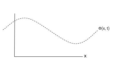
Now that we have a way to express our theories, we need to figure out a way to represent the building blocks of a theory. We could use particles as the building blocks, and represent each particle by its position and velocity. However, fields turn out to be a much more useful way of representing the way particles behave. A field $\phi(x, t)$ is a function that takes a point in spacetime and spits something out for each point.

For example, a field could take a position (in spacetime) and spit out a number (which could be real or complex). Or it could also take a position and output a vector. It turns out that we can describe the way fields evolve - so the numbers or vectors or whatever assigned to each position in spacetime - using the same mechanism we used for particles. We take the field at each point in spacetime, apply some Lagrangian to it to get a number, and add that number for all points in spacetime. Then, the field will evolve in a way that minimizes the Lagrangian.

In practice we don’t actually try to predict the motion of a field or particle by taking the Lagrangian of our theory and summing it up for every possible path. Instead we use a set of equations, known as the Euler-Lagrange equations, that allow us to derive the equations of motion for a given Lagrangian. However, we won’t need those equations for now - we’ll just work with the Lagrangian.

Let’s say we have some complex field $\phi$. Just to keep things as simple as possible, let’s say that the field is only a function of time. The simplest Lagrangian we can write for this field is:

\[\mathcal{L} = \delta_t\phi^\star \delta_t\phi\]

The $\delta_t\phi^\star \delta_t\phi$ term represents the kinetic energy of the field (which is the energy associated with the motion of the field). Also note that intead of squaring the field, we’re multiplying it by its complex conjugate. This isn’t strictly necessary in this case [4], but since it’s required for fields that describe many of the particles in the Standard Model, we’ll use it here to make this model more realistic.

One interesting observation about Lagrangians is that any term of the form $V(\phi)$ represents potential energy. Since there are no time or space derivatives involved, the term indicates the influence of the ‘position’ of the field itself, instead of the effects of how its changing in space or time (which would represent kinetic energy).

Gauge Invariance

We’re now ready to start discussing symmetry, and how it affects our theory.

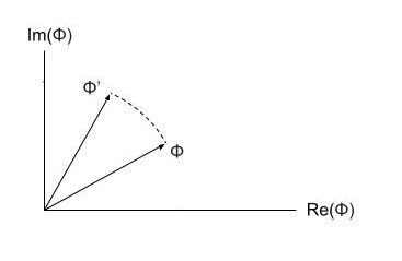
Let’s try to see what happens to the Lagrangian if we ‘rotate’ our field. Since the field is complex, and complex numbers are just points on the 2D plane, we should be able to go to every point in the field and just rotate it by some amount. To rotate a complex number, we multiply it by $e^{i\theta}$ where $\theta$ is some angle, which means that our field $\phi$ will turn into $e^{i\theta}\phi$, and its complex conjugate $\phi^\star$ will become $e^{-i\theta}\phi^\star$.

But what does this rotation do to our Lagrangian? This is an important question since the Lagrangian is what generates the equations of motion for our theory, so if the rotation affects the Lagrangian, it means that it’ll have some effect on the theory itself. But interestingly, note that the rotation leaves the Lagrangian unchanged! If we take the derivatives:

\[\delta_t\left[e^{i\theta}\phi\right] = e^{i\theta}\delta_t\phi\] \[\delta_t\left[e^{i\theta}\phi\right]^\star = e^{-i\theta}\delta_t\phi^\star\]

The $e^{i\theta}$ and $e^{-i\theta}$ terms cancel out, leaving the Lagrangian the same. This makes some sense intuitively - if two people decide to ‘measure’ complex numbers differently, with one person using a coordinate system that’s rotated relative to the other, this shouldn’t change what they observe.

Now let’s take this a step further. In the previous example, we rotated the field at all points by some angle. But why do we need to rotate the field the same way everywhere? What if we measure things at one point with one coordinate system, but measure them at a different point using a different coordinate system that’s rotated. Although it’s hard to imagine why anyone would want to do this, one would still expect that this shouldn’t affect the actual physics predicted by the theory. So instead of using $\theta$ like we did earlier, we’ll now use a function $\theta(t)$.

The Lagrangian involves derivatives of the fields, so let’s take derivatives.

\[\delta_t\left[e^{i\theta(t)}\phi\right] = \left[\delta_t\phi +i\phi\frac{\delta\theta}{\delta t}\right]e^{i\theta(t)}\] \[\delta_t\left[e^{i\theta(t)}\phi\right]^\star= \left[\delta_t\phi^\star -i\phi^\star\frac{\delta\theta}{\delta t}\right]e^{-i\theta(t)}\]

Multiplying these together, we see that the Lagrangian is different. This is not what we wanted - rotating the complex plane in has affected the results of our theory.

So how do we fix this? Note that the issue here is that when we take the derivative of the field, we get an extra $i\phi\frac{\delta\theta}{\delta t}$ term proportional to the derivative. To remove this term, we need something else that, when transformed, results in the exact same term but with opposite sign. To do this, we add a new field $A$ to our Lagrangian and say that when the complex plane is rotated, this field transforms in a way that produces that exact term that we need to cancel out.

\[A' = A + \delta_t\theta\]

Our new Lagrangian is:

\[\mathcal{L} = \delta_t\phi^\star \delta_t\phi + iA\phi\]

This property - that a theory is not affected by changing some symmetry parameter throughout spacetime - is called gauge invariance. Note that we were able to take a theory that was not gauge invariant, but made it gauge invariant by adding another field. Also note that this new term, $iA\phi$, looks like a potential from the perspective of our field, with $V(\phi) = iA\phi$, and since potentials represent forces, our theory now predicts some type of force involved in the interaction between our field and this new field.

This mechanism of introducing an additional field to make an existing theory gauge invariant is exactly what gives rise to photons in the Standard Model! ‘Rotations’ of the electron field correspond to an additional field, called a gauge field, that behaves exactly the way photons do.

Let’s try to take a closer look at where this field comes from. There’s an interesting geometric way to look at this field. Going back to our original Lagrangian, note that we’re trying to take derivatives of our field. A derivative is really just a difference (using $x$ instead of $t$ now):

\[\delta\phi(x) = \lim_{\delta x \rightarrow 0}{\frac{\phi(x + \delta x) - \phi(x)}{\delta x}}\]

This derivative doesn’t really make sense if we aren’t using the same coordinate system everywhere. The way we measure our field at $x$ is different than the way we measure it at $x + \delta x$, so to get the actual difference, we need to make the field comparable by fixing it up before subtracting it. Let’s define a function $W(x, y)$ that takes the field at $y$ and ‘fixes it up’ so that it can be compared to the field at $x$. With this function, we can come up with a new definition of a derivative - called the covariant derivative:

\[D\phi(x) = \lim_{\delta x \rightarrow 0}{\frac{W(x, x + \delta x)\phi(x + \delta x) - \phi(x)}{\delta x}}\]

Can we learn anything about this function $W$? As a first step, we can expand it:

\[W(x, x + \delta x) = 1 - i\delta xA(x) + \mathcal{O}(\delta x^2)\]

Note that the first term will be $1$ since if $\delta x$ is zero, we want the function to not change the field. I’ve labelled the coefficient of the linear term $A(x)$, and since $\delta x$ is small, we can leave out higher order terms. Plugging this back into the definition of the covariant derivative, we see that the derivative becomes:

\[D\phi(x) = \delta\phi + iA\phi\]

Which contains the exact term that we added to our Lagrangian to make it gauge invariant. This shows that the new field is a tool that allows us to sensibly take the derivative of our field.

Groups and Other Symmetries

So far, we’ve considered the implications of having a theory that is symmetric in terms of rotations - we’re allowed to rotate individual fields. But we can go further - what if our theory contained different types of fields, but was symmetric in terms of rotations across these fields. For example, suppose you have a model where you have two fields, $\phi_1$ and $\phi_2$. You make an observation - that some particle exists in $\phi_1$, but none in $\phi_2$. In a way, $\phi_1$ and $\phi_2$ are being used as coordinates - you specify your observation of some particles by stating which fields they are represented by.

However, another observer may be using a set of coordinates (or fields) that are ‘rotated’ relative to yours. So a particle that you consider to be in $\phi_1$ might be represented by $-\phi_2$ for them, and a particle represented by $\phi_2$ could be represented by $\phi_1$ in their case. This is hard to visualize since complex numbers are involved, but the idea is just that we’re performing rotations in a space with multiple fields.

It turns out that there are a range of particles in nature that exhibit this kind of symmetry. There isn’t any easy way to argue why this kind of symmetry must exist, but it does - so let’s explore some of its consequences on the theory. But first, some terminology.

The symmetry we considered earlier, involving the rotation of complex numbers by some angle, is called a $U(1)$ symmetry. This term comes from group theory, and more specifically the idea of a representation. A group is a set of elements associated with some operation. So in our case, each group element is a rotation. But we can also represent each rotation by a matrix, specifically a $1 \times 1$ matrix of length $1$: $\left[e^{i\theta}\right]$.

What’s important here is that these two sets - the set of rotations, with the operation being composition, and the set of $1 \times 1$ complex matrices with the operation being multiplication - have the exact same behavior, i.e., you can map rotations from the first set to $1 \times 1$ matrices from the second set in a way that if you perform a group operation on elements in the first set, you get the corresponding element in the second set.

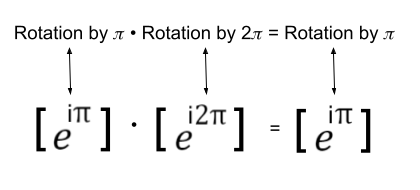
This provides us a convenient way to label symmetry operations. Rotations in the complex plane correspond to multiplication of $1\times1$ matrices, and since the group of $1 \times 1$ matrices of magnitude 1 is called $U(1)$, we refer to our symmetry as a $U(1)$ symmetry (the U stands for unitary, which are complex matrices that preserve lengths and angles). It turns out that the group of rotations where two different complex fields are rotated can be represented by $2 \times 2$ unitary matrices and is called $SU(2)$ [5]. The group of rotations where three different fields are rotated can be represented by $3 \times 3$ unitary matrices, and is called $SU(3)$.

Earlier, we tried making a $U(1)$ transformation to our Lagrangian and found that an additional field becomes necessary as a result of this symmetry. If we have two fields in our Lagrangian that have $SU(2)$ symmetry (i.e., they can be rotated), is that automatically gauge invariant? Or do we need to add more fields as well, just like we had to in the $U(1)$ case?

We still have the same problem as before - we can’t compare fields at neighboring points when taking the derivative, since the definition of each field is different - it is rotated at different points. Again, we introduce a field $A$ that helps us compare fields at different points.

Now what exactly is $A$ doing? It’s modifying our field in a way that undoes the changes in the symmetry parameter - so it also represents a symmetry transformation. An important observation is that symmetry operations can generally be broken down into smaller, more fundamental operations. For example, consider the group of rotations in three dimensions. Each small rotation in three dimensions can be written as the sum of a small rotation along the $x$ axis, a small rotation along the $y$ axis, and a small rotation along the $z$ axis. These smaller rotations are called generators of the rotation group.

We can use the idea of generators to write $A$ as a sum:

\[A = \sum_{a}A^aT^a\]

Where $T^a$ are the different generators.

The key insight here is that $A$ can be broken down into multiple fields, one per generator, indicating how much of that generator needs to be used.

If we interpret fields as particles, then this implies that if our Lagrangian is to be gauge invariant under some symmetry group, then we must add more fields (or particles) - one for each generator of that symmetry group. And this is exactly what we see in the Standard Model:

• $U(1)$ invariance of the electron field gives rise to the photon field.
• $SU(2)$ invariance across lepton fields (such as the electron and electron neutrino) leads to $W^+$, $W_-$, and $Z$ bosons. $SU(2)$ has two generators, so there are three gauge bosons.
• $SU(3)$ invariance across quark fields leads to eight gluons, since $SU(3)$ has eight generators.

This is the sense in which $ U(1) \times SU(2) \times SU(3) $ is said to be the symmetry group of the Standard Model, as the Lagrangian for the Standard Model is invariant under the symmetry transformations represented by these groups. It’s remarkable how the observation that an equation doesn’t change under some operation, which seems quite trivial, can have deep consequences, dictating the nature of forces and interactions in the theory.

Notes

[1] Symmetry won’t tell you every particle that exists, but it can be used to infer the presence of certain particles, as discussed here.

[2] All particles are representations of the Lorentz group.

[3] Noether’s theorem links each symmetry to a conservation law.

[4] In technical terms, we’re able to construct a Lorentz invariant Lagrangian for spin 0 fields without using the complex conjugate.

[5] The S stands for special, and it means that the matrices must have determinant 1.